Euler-Lagrange Equation
Lagrangian Mechanics
Compared to Newtonian mechanics, Lagrangian Mechanics presents an alternative perspective on how to analyze physics problems.
The Lagrangian \(\mathcal{L}\) and Euler-Lagrange Equation
Let’s start with some definitions.
The lagrangian is defined as \(\mathcal{L} = T - U\), where \(T\) is the kinetic energy of the system and \(U\) is the potential energy of the system.
The Euler-Lagrange equation is given by
\[\frac{d}{dt}\left(\frac{\partial \mathcal{L}}{\partial \dot{x}}\right) - \frac{\partial \mathcal{L}}{\partial x} = 0\]Let’s use this to analyze a few problems
Falling object
Suppose we have a still object that falls subject to just gravity.
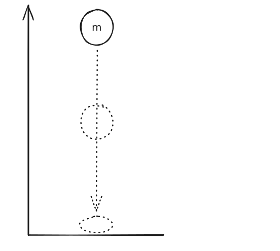
- The coordinate frame starts at \(0\) from the ground up to \(x_0\), the starting height of the object.
- The object has mass \(m\) and falls under the influence of gravity.
Now let’s compute the lagrangian \(\mathcal{L}\).
(We use dot notation to denote derivatives of \(x\) with respect to time. i.e. velocity and acceleration.)
Using this, we now apply the Euler-Lagrange equation.
\[\frac{d}{dt}\left(\frac{\partial \mathcal{L}}{\partial \dot{x}}\right) - \frac{\partial \mathcal{L}}{\partial x} = 0\]Computing each term one-by-one gets us the following:
\[\frac{\partial\mathcal{L}}{\partial x} = -mg\] \[\frac{\partial\mathcal{L}}{\partial \dot{x}} = m\dot{x}\] \[\frac{d}{dt}\left(\frac{\partial\mathcal{L}}{\partial \dot{x}}\right) = m\ddot{x}\]Thus, we have the following
\[\frac{d}{dt}\left(\frac{\partial \mathcal{L}}{\partial \dot{x}}\right) - \frac{\partial \mathcal{L}}{\partial x} = m\ddot{x} - (-mg) = 0\]This reduces to
\[\ddot{x} = g\]From this, we derive the following equation for the object with respect to time, which matches what we expect from Newtonian mechanics.
\[x(t) = -\frac{1}{2}gt^2 + v_0t + x_0\]Springs
Consider an object with mass \(m\) attached to a spring following ideal spring properties.
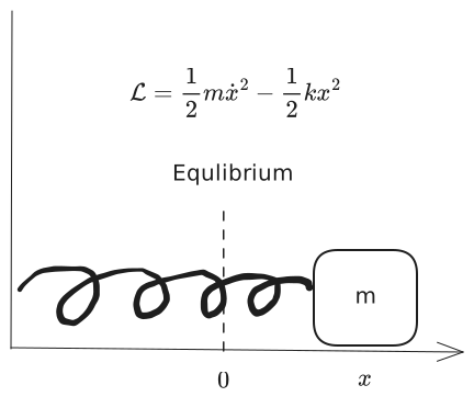
As before, we compute the lagrangian and terms of the Euler-Lagrange equation:
\[\mathcal{L} = \frac{1}{2}m\dot{x}^2 - \frac{1}{2}kx^2\] \[\frac{d}{dt}\left(\frac{\partial \mathcal{L}}{\partial \dot{x}}\right) - \frac{\partial \mathcal{L}}{\partial x} = 0\]The terms are the following:
\[\frac{\partial \mathcal{L}}{\partial x} = -kx\] \[\frac{\partial \mathcal{L}}{\partial \dot{x}} = m\dot{x}\] \[\frac{d}{dt}\left(\frac{\partial \mathcal{L}}{\partial \dot{x}}\right) = m\ddot{x}\]Thus we have the following:
\[\frac{d}{dt}\left(\frac{\partial \mathcal{L}}{\partial \dot{x}}\right) - \frac{\partial \mathcal{L}}{\partial x} = m\ddot{x} - (-kx)= 0\]This reduces to
\[\ddot{x} + \frac{k}{m}x = 0\]From this, we know the solution has the following form, which we expect intuitively from an object oscillating from the force of a spring.
\[x(t) = A\cos(\omega t)\]Calculus of Variations
Let’s review a bit what we know from basic calculus. From calculus, we already know how to solve for local minimas/maximas. For some function \(f(x)\), we solve for the solutions of the equation: \(f'(x) = 0\). After obtaining solutions to this equation, we use other techinques like the second derivative to determine what kind of stationary point we’ve found.
In calculus of variations, we extend this concept with one more layer of indirection.
Instead of searching for stationary points, we search for stationary functions: functions \(f\) that minimizes or maximizes some quantity \(I[f]\).
Analytically, we are trying to min/max the quantity \(I[f] = \int_{x_1}^{x_2} F(x, y, \frac{dy}{dx}) dy\) for some \(F(x, y, \frac{dy}{dx})\).
(Note: \(F(x, y, \frac{dy}{dx})\) can possibly take more parameters, but we restrict our attention to these parameters now.)
Let’s move to derive the Euler-Lagrange equation.
We have some \(F(x, y, \frac{dy}{dx})\) defined and are trying to optimize \(I[f] = \int_{x_1}^{x_2} F(x, y, \frac{dy}{dx}) dy\). Suppose also that a \(y(x)\) exists that makes \(I\) stationary. We also start already knowing the values \(y(x_1)\) and \(y(x_2)\). So, we introduce \(\eta(x)\) where \(\eta(x_1) = \eta(x_2) = 0\) and define \(\bar{y}(x) = y(x) + \epsilon\eta(x)\).
Our goal is to find \(\bar{y}(x)\) that makes \(I(\epsilon) = \int_{x_1}^{x_2} F(x, \bar{y}, \bar{y}') dx\) stationary.
Since \(y\) is assumed to be stationary and \(I\) only depends on \(\epsilon\), \(\left. \frac{dI}{d\epsilon} \right\vert_{\epsilon=0} = 0\)
We have the following sequence of computation:
\[\begin{align} \left.\frac{d}{d\epsilon}\right\vert_{\epsilon=0}\int_{x_1}^{x_2} F(x, \bar{y}, \bar{y}')dx &= 0 \\ \left.\int_{x_1}^{x_2} \frac{d}{d\epsilon} F(x, \bar{y}, \bar{y}')\right\vert_{\epsilon=0}dx &= 0 \\ \left.\int_{x_1}^{x_2} \left[ \frac{\partial F}{\partial\bar{y}}\frac{\partial\bar{y}}{\partial\epsilon} + \frac{\partial F}{\partial\bar{y}'}\frac{\partial\bar{y}'}{\partial\epsilon} \right] \right\vert_{\epsilon=0}dx &= 0 \text{ (Only } y \text{ depends on } \epsilon\text{)}\\ \left.\int_{x_1}^{x_2} \left[ \frac{\partial F}{\partial\bar{y}}\eta + \frac{\partial F}{\partial\bar{y}'}\eta' \right] \right\vert_{\epsilon=0}dx &= 0 \text{ (Definition of }\bar{y}\text{)} \\ \left.\int_{x_1}^{x_2} \left[ \frac{\partial F}{\partial\bar{y}}\eta - \frac{d}{dx}\frac{\partial F}{\partial\bar{y}'}\eta \right] \right\vert_{\epsilon=0}dx &= 0 \text{ (integration by parts)}\\ \left.\int_{x_1}^{x_2} \left[ \frac{\partial F}{\partial\bar{y}} - \frac{d}{dx}\frac{\partial F}{\partial\bar{y}'} \right]\eta \right\vert_{\epsilon=0}dx &= 0 \\ \int_{x_1}^{x_2} \left[ \frac{\partial F}{\partial y} - \frac{d}{dx}\frac{\partial F}{\partial y'} \right]\eta dx &= 0 \\ \end{align}\]Since \(\eta\) was arbitrary, the equation is true only when the Euler-Lagrange equation \(\frac{\partial F}{\partial y} - \frac{d}{dx}\frac{\partial F}{\partial y'} = 0\) is satisfied.
From our derivation, the Euler-Lagrange equation is a necessary condition for stationary functions, but not sufficient.