Explaining PCA

Principle Component Analysis

Principle Component Analysis (PCA) is a fancy terms for a technique used in reducing the dimension of multi-dimensional data while maximizing the variance of the data. Here, we explore the geometric meaning behind PCA.

Example with Python

from sklearn.decomposition import PCA
from sklearn.datasets import load_digits
import matplotlib.pyplot as plt
%matplotlib inline

We can go through an example of PCA with python.
Here, we are using the digits dataset provided in sklearn.
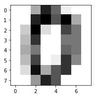
Each datapoint is an 8x8 image, which can be thought as a single point in 64 dimensional space.
Let’s take a look at what a data point looks like.

digits = load_digits()
plt.figure(figsize=(3,3));
plt.imshow(digits.images[0], cmap=plt.cm.gray_r);

digits.data.shape

(1797, 64)

The actual data can be modelled by a 1797x64 matrix where each row is an individual data point.
Let’s run the data through PCA.

pca = PCA(n_components=2)
pca.fit(digits.data)
values = pca.transform(digits.data)

plt.figure(figsize=(10,8))
plt.scatter(values[:, 0], values[:, 1], c=digits.target, s=30,
            alpha=0.7, cmap=plt.cm.get_cmap('tab10', 10));
plt.colorbar();

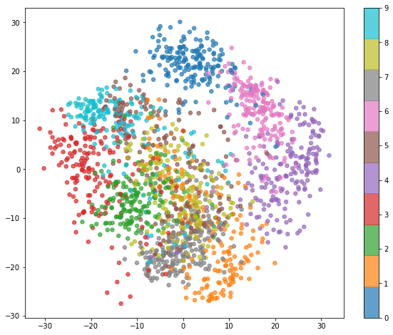
From the photo, we see that numbers 0, 4, and 6 all seem to be easily separable from all the other datapoints.
Numbers, such as 1 and 7 seem to be hard to separate.

The Multivariate Gaussian

The multivariate gaussian distribution is a generalization of the 1-dimensional gaussian distribution to multiple distribution.
The equation for the n-dimensional distribution is

\[p(x;\mu,\Sigma) = \frac{1}{(2\pi)^{n/2}|\Sigma|^{1/2}} exp(-\frac{1}{2}(x-\mu)^\top \Sigma^{-1}(x-\mu))\]

Here, \(\mu\) is a vector and \(\Sigma\) in the covariance matrix of the distribution.

The key to understanding the multi-variate gaussian distribution is the covariance matrix \(\Sigma\). \(\Sigma\) is a positive-definite symmetric matrix where the value at the \((i, j)\) position is the covariance between the \(i\) component and \(j\) component of the distribution.

Since \(\Sigma\) is symmetric and positive-definite, its inverse \(\Sigma^{-1}\) is also. Then, every eigenvector of \(\Sigma\) is also an eigenvector of \(\Sigma^{-1}\) and for every eigenvalue \(\lambda\) of \(\Sigma\), \(\frac{1}{\lambda}\) is an eigenvector of \(\Sigma\).
Being symmetric, we can find a set of orthornormal eigenvectors of \(\Sigma\), \(\{v_1, \ldots, v_n\}\) that span the whole space. Thus, we can diagonalize the matrix \(\Sigma^{-1}\) as:

\(\Sigma^{-1} = \begin{bmatrix} | & \cdots & | \\ v_1 & \cdots & v_n \\ | & \cdots & | \end{bmatrix} \begin{bmatrix} \frac{1}{\lambda_1} & 0 & \cdots & 0 \\ 0 & \frac{1}{\lambda_2} &\cdots & \vdots \\ \vdots & \vdots & \ddots & \vdots \\ 0 & \cdots & \cdots & \frac{1}{\lambda_n} \end{bmatrix} \begin{bmatrix} - & v_1^{\top} & - \\ \vdots & \vdots & \vdots\\ - & v_n^{\top} & - \end{bmatrix}\)
At the beginning, we have \(x^\top\Sigma^{-1}x\) in the argument of the exponential. (Here, I’m assuming \(\mu\) is 0).
It turns out \(x^\top\Sigma^{-1}x\) is a quadratic form that describes some ellipsoid. If we diagonalize \(\Sigma^{-1}\), we can obtain \(x^\top Q\Lambda Q^\top x\). In this form, we see that \(Q\) and \(Q^\top\) act as rotations on vectors while \(\Lambda\) scales the vectors.
If we take level curves by finding all values of \(x\) that satisfies the equation \(c = x^\top Q\Lambda Q^\top x\), we obtain an ellipsoid whose axis are determined by the orthornormal vectors: \({v_1,\ldots, v_n}\).
The lengths of the axes determined by each \(v_i\) proportional with \(\sqrt{\lambda_i}\).

Suppose we have the covariance matrix \(\Sigma=\begin{bmatrix} 4 & 0 \\ 0 & 9 \end{bmatrix}\). According to our analysis, we expect the multivariate gaussian distribution to have axes aligned with the standard cartesian axes, and the level curves to form an ellipse where the axis are in a \(2:3\) ratio.

\[x^\top\Sigma^{-1}x = \begin{pmatrix}x_1 & x_2\end{pmatrix} \begin{bmatrix}\frac{1}{4} & 0 \\ 0 & \frac{1}{9} \end{bmatrix} \begin{pmatrix}x_1 \\ x_2\end{pmatrix}\]

Taking level curves of this quadratic form, we obtain \(\frac{x_1^2}{4} + \frac{x_2^2}{9} = c\), which is the equation for an ellipse that carries these exact properties.

Back to PCA

PCA attempts to project some amount of data onto a smaller dimensional space that best represents the bigger space. In other words, PCA finds an orthogonal set of vectors such that projecting the data points onto its linear span will capture the most variance.
Given the covariance matrix of the data, we have all the data we need to determine the principle components. From our study of the multivariate gaussian, we know that the vector that best best fits the data is an eigenvector of the covariance matrix with the largest eigenvalue. Similarly, the best 2-dimensional plane that fits the data is the span of the two eigenvectors that have the two largest eigenvalues. In this way, we can find any \(k\) eigenvectors whose span best captures the variance of the data.

Using SVD to perform PCA

The above analysis gives us a way to compute the principle components of some set of data. We simply diagonalize the covariance matrix and project everything onto the span of the \(k\) eigenvectors with the largest eigenvalues.

However, another way to approach this would be to use Singular Value Decomposition (SVD). SVD is a way to factor any matrix \(A\) into the product of 3 lower rank matriecs, \(U\Sigma V^\top\). (Note that the \(\Sigma\) here is different from the \(\Sigma\) from earlier.) \(U\) is the matrix of eigenvectors of \(A^\top A\) and \(V\) is the matrix of
eigenvectors of \(AA^\top\).
\(\Sigma\) is a diagonal matrix that contains the squareroots of the eigenvalues of both \(A^\top A\) and \(AA^\top\).

Suppose we have a matrix \(X\) that contains our data where each row represents a data point and the columns represent the features. For practical purposes, we will assume that each feature is centered at 0 and already normalized.
Then, the covariance matrix is simply \(X^\top X\).
If we perform SVD on \(X\), we obtain \(X = U\Sigma V^\top\). Notice that for the covariance matrix, \(X^\top X = V\Sigma^2V^\top\). By performing SVD on \(X\), we are also finding the eigenvectors and eigenvalues of the covariance matrix \(X^\top X\).
We also obtain the coefficients for each data point in terms of the eigenvectors in \(V\) with \(U\Sigma\). This can be seen in \(X = (U\Sigma)V^\top\) or the equation: \(x_i = \sum_{j=1}^k U_{i,j}\Sigma_{j,j}v_j \).

Thus, by using SVD, we can obtain the vectors whose linear span best captures the variance of the data, and find the coefficients of the data points when projected onto the span.